Neural Scaling Laws

Inverted CERN School of Computing - iCSC 2026

Albert Sund Aillet

Presentation: albert.sundaillet.com/scaling-laws

About the Speaker

Research/Software Engineer at CERN.

Participated in main CSC 2025, Lund

Education:

BSc Engineering Physics, KTH (Stockholm, Sweden).
MSc Machine Learning, KTH and EPFL (Lausanne, Switzerland).

Summary of Talk

Brief history of AI
Neural networks and training
Language models
Transformers and attention
Scaling laws and why they matter
Different scaling axes
Future outlook

A Brief History of Artificial Intelligence

The field of artificial intelligence has evolved significantly since its inception in the 1950s.

Two major paradigms:

Symbolic AI

Top-down, logic-based

Connectionism

Bottom-up, biologically inspired

Symbolic AI

Origins: Dartmouth Conference, 1956 - high-level reasoning and knowledge representation
Core idea: intelligence as symbol manipulation and logic (top-down)
Peak: Expert Systems of the 1980s - massive "if-then" rule databases
Strengths: formal logic, arithmetic, transparency, interpretability
Weakness: brittle - couldn't handle ambiguity, perception, or commonsense reasoning

Symbolic AI in Practice: ELIZA (1966)

Early chatbot using pattern matching and scripted rules.

Coined the ELIZA effect: people attribute human-like understanding to computer programs.

Anthony Hay, Joseph Weizenbaum's 1966 ELIZA recreated https://github.com/anthay/ELIZA

Wikipedia Contributors, ELIZA https://en.wikipedia.org/wiki/ELIZA

Connectionism

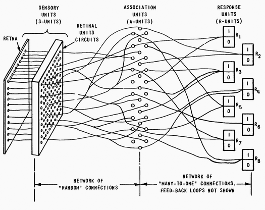
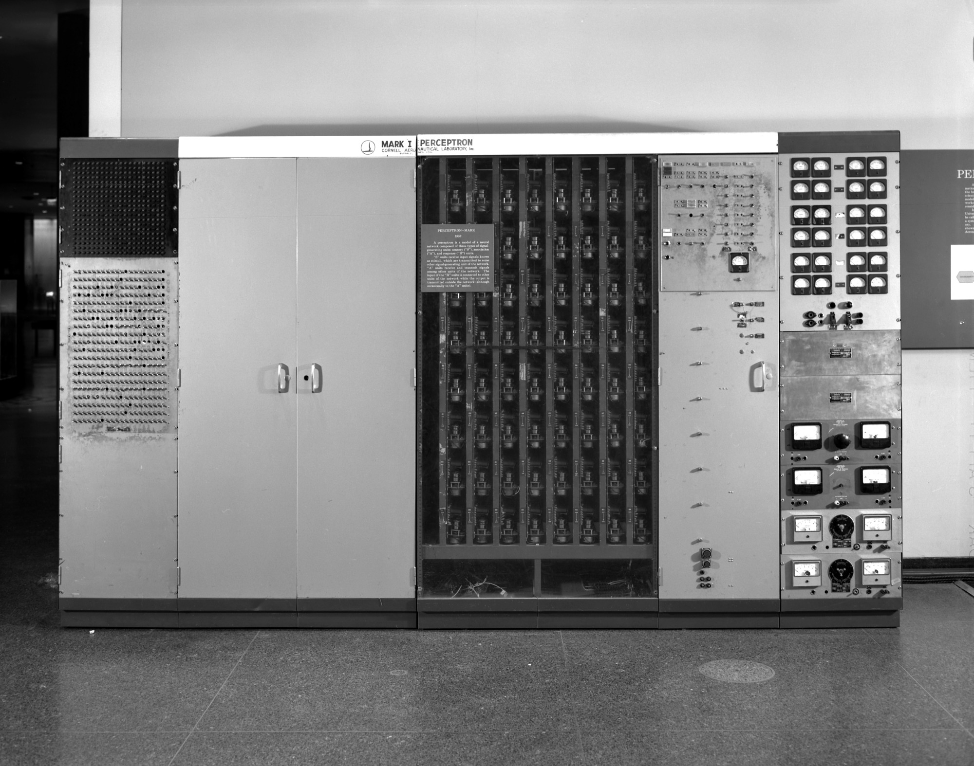
Origins: Rosenblatt's Perceptron (1957)
Designed to mimic biological neurons
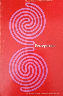
1969: Minsky & Papert showed limits of single-layer perceptrons, contributing to the first AI winter
Revival: backpropagation in the 1980s enabled training of multi-layer networks
Strength: excels at perception, language, and tasks that resist explicit rules
Weakness: requires large amounts of data and compute and is not easily interpretable

Hay et al., Organization of the Mark I Perceptron Figure 1, p. 13

The Perceptron (1957)

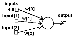
Frank Rosenblatt's Perceptron introduced a learnable neuron model
Key idea: learn weights from data rather than hand-crafted rules
Influential early milestone in neural network history

Minsky and Papert, (1969) Perceptrons: An Introduction to Computational Geometry wikipedia.org

Neural Networks

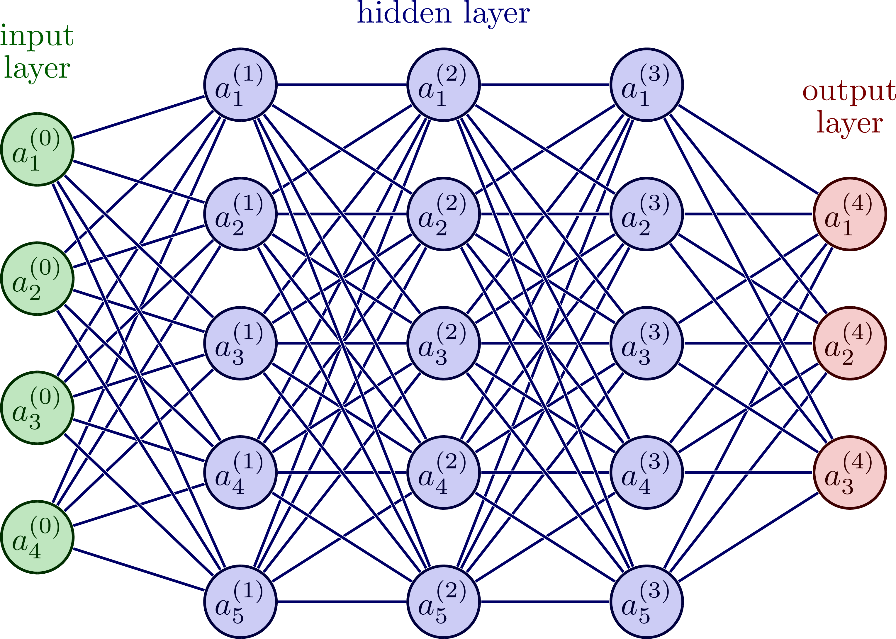
Neural networks are composed of interconnected nodes (neurons) organized in layers
Each connection has a weight that is adjusted during training
Activation functions introduce non-linearity into the model

\[ \mathbf{a}^{(l+1)} = \sigma \left( \mathbf{W}^{(l+1)} \mathbf{a}^{(l)} + \mathbf{b}^{(l+1)} \right) \]

Diagram of a simple feedforward neural network — A simple feedforward neural network.

Loss Functions

A loss function measures how far predictions are from targets
Training minimizes the average loss over the dataset
For language modeling, the standard choice is cross-entropy

\[ L = - \frac{1}{T} \sum_{t=1}^{T} \log p(x_t \mid x_{\lt t}) \]

Backpropagation (Forward + Backward)

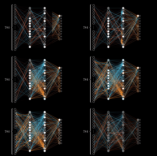
Forward pass: compute predictions and the loss
Backward pass: apply the chain rule to compute gradients
Gradients tell us how to update weights to reduce the loss
1980s revival: backpropagation enabled training of multi-layer networks
Scale + data + compute drove modern performance leaps

\[ \nabla_{\theta} L = \frac{\partial L}{\partial a} \cdot \frac{\partial a}{\partial \theta} \quad \text{where } \theta \text{ is model parameters and } L \text{ is the loss} \]

Backpropagation animation from NVIDIA's Data Scientist's Guide to Backpropagation

Jürgen Schmidhuber, Who Invented Backpropagation? people.idsia.ch/~juergen/

Rumelhart, Hinton, Williams (1986), Learning representations by back-propagating errors nature.com

Stochastic Gradient Descent

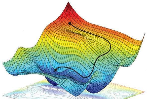
SGD updates model parameters in the direction of the negative gradient
Mini-batches are used to approximate the full gradient
Adam is a popular variant that adapts the learning rate for each parameter

\[ \theta \leftarrow \theta - \eta \, \nabla_{\theta} L \]

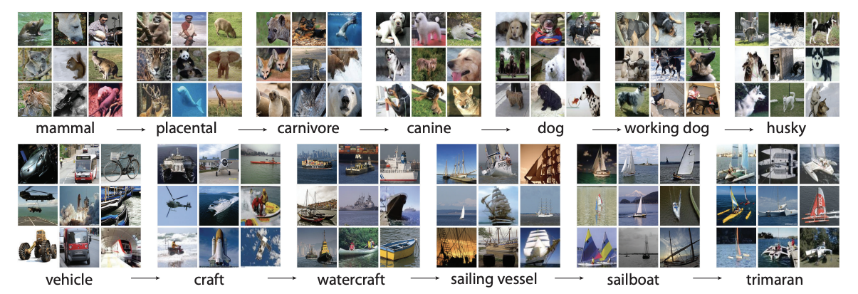
ImageNet

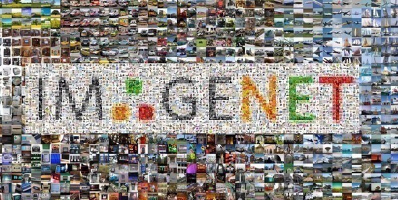
ImageNet: a large labeled image dataset (14M images, 1,000 classes) used as a benchmark for visual recognition
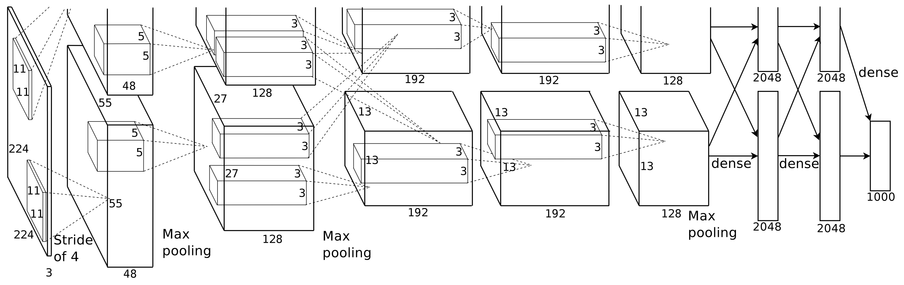
Deep convolutional network approaches dramatically improved ImageNet accuracy
Marked the beginning of the modern deep learning era
The entire field of computer vision moved to deep learning
Trained on 2 Nvidia GTX 580 GPUs

Deng, et al. (2009) ImageNet: A Large-Scale Hierarchical Image Database imagenet.org

Krizhevsky, Sutskever, Hinton (2012), ImageNet Classification with Deep Convolutional Neural Networks NeurIPS paper

Cireșan, Meier, Schmidhuber (2012), Multi-column Deep Neural Networks for Image Classification arXiv:1202.2745

What is a Language Model?

A language model is a type of neural network trained to predict the next token in a sequence of text
It learns statistical patterns and structures in language, enabling it to generate coherent text

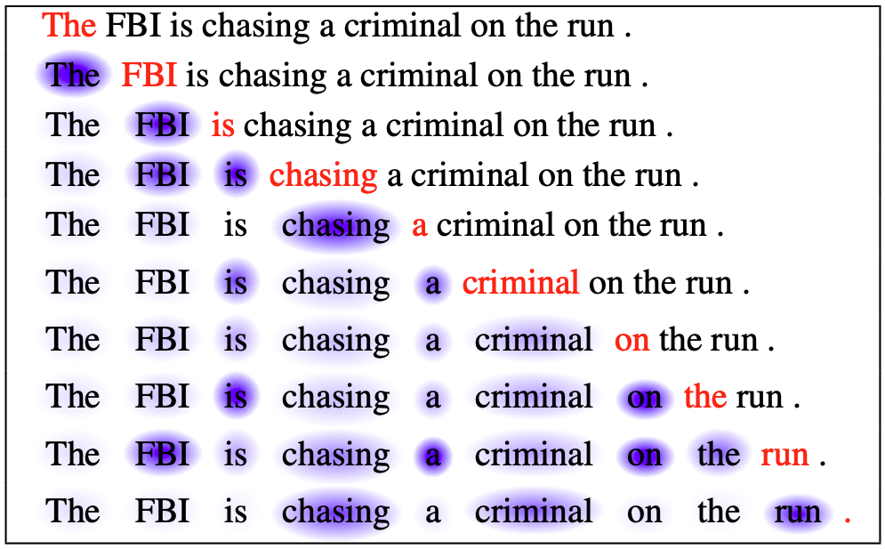
Diagram of autoregressive language modeling — Autoregressive language modeling - each token conditions on all prior tokens

Why focus on language modeling?

Human language is an efficient system for encoding information about the world
Huge volumes of text are freely available online, approximately 10 million books in the Library of Congress containing roughly 1 trillion words
An AI with language proficiency can be queried on any topic, providing significant insight into its capabilities (compare to predicting protein structures or Go moves)

Library shelves representing large text corpora

Tokenization

Text is broken into sub-word units called tokens, not raw characters or whole words
Example: "unbreakable" → "un" + "break" + "able"
Common algorithm: Byte-Pair Encoding (BPE) - merges frequent character pairs iteratively
Each token is a number (a token ID) the model looks up in an embedding table
Tokenization is a source of subtle model behavior (arithmetic, rare words, languages)

Autoregressive Language Modeling

Model language by predicting the next token in a sequence

\[ P(\text{token}_t \mid \text{token}_{t-1}, \ldots, \text{token}_{1} ) \]

Maximize likelihood of the training corpus
At inference time, tokens are sampled one at a time - each prediction conditions on all prior tokens

Cheng, Dong, Lapata (2016) Long Short-Term Memory-Networks for Machine Reading arXiv:1601.06733

Embedding Space

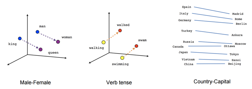
Tokens are mapped to dense vectors in a high-dimensional embedding space
Geometry encodes meaning: similar words cluster together
These representations are learned end-to-end during training

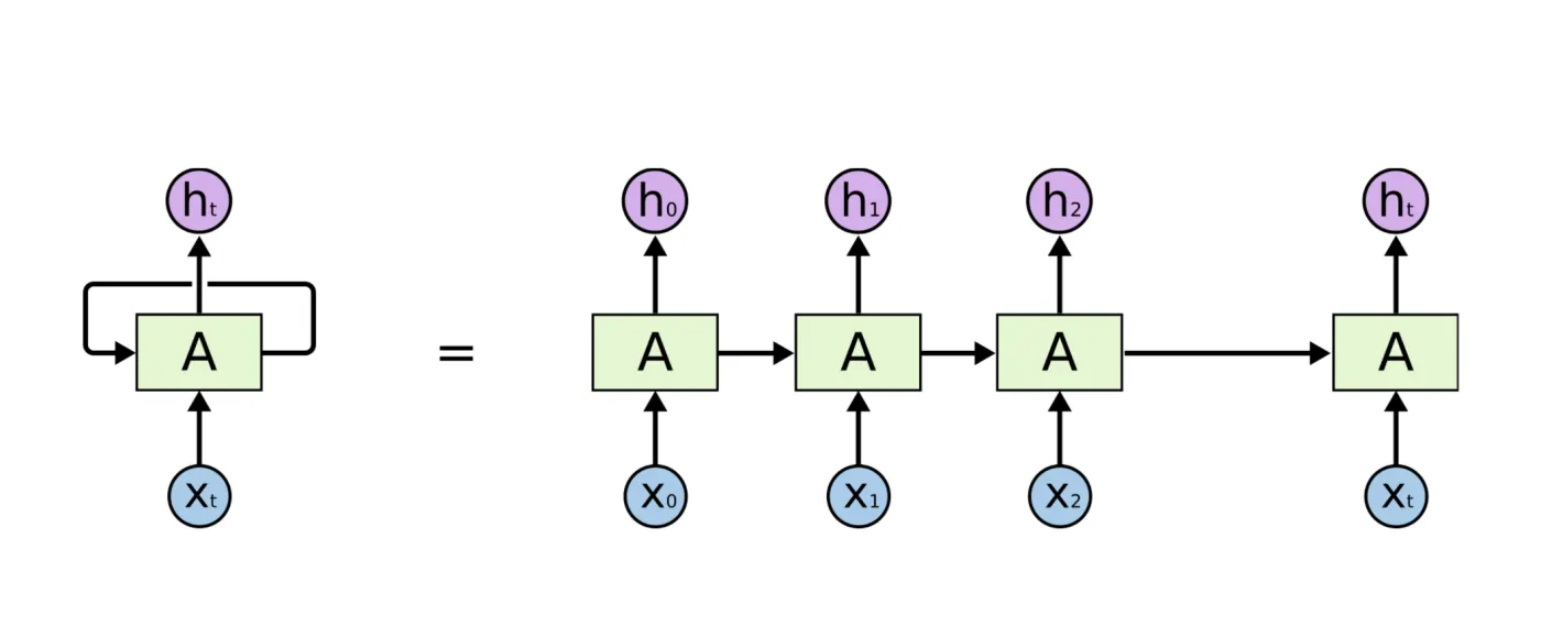
Limitations of RNNs and LSTMs

Sequential processing makes training and inference slower
Vanishing/exploding gradients over long sequences
Backpropagation Through Time is costly and hard to scale
Long-range dependencies are difficult to capture reliably

Transformer Neural Network Architecture

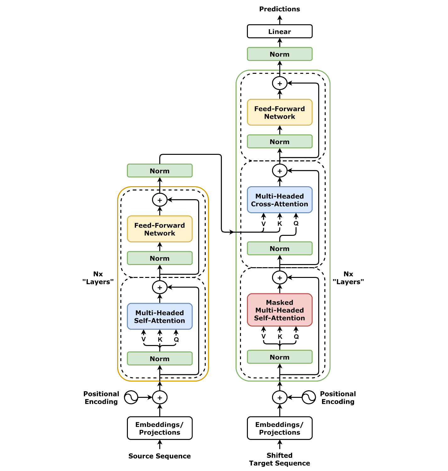
Transformer (Vaswani et al. 2017): stacked self-attention and feed-forward blocks (with residual connections)
GPT-type models are decoder-only: each token attends to all previous tokens

Vaswani et al., Attention Is All You Need, arXiv:1706.03762 (2017)

Parikh et al., A Decomposable Attention Model for Natural Language Inference, arXiv:1606.01933 (2016)

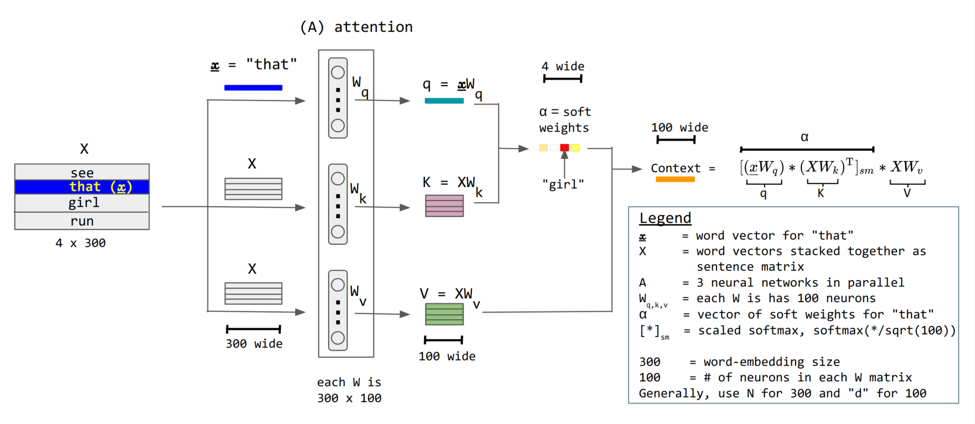
Self-Attention Intuition

Each token builds a weighted summary of earlier tokens
Weights come from learned queries and keys
Parallel attention replaces sequential recurrence
Stack many layers to build deeper representations

Diagram of attention mechanism showing queries, keys, and values

Attention diagram from wikipedia.org

What Is a Scaling Law?

\[ y = a \, x^{b} \quad\Longleftrightarrow\quad \log y = b \log x + \log a \]

A scaling law is a mathematical relationship between two quantities where one quantity varies as a power of another
Scaling laws hold across many orders of magnitude and are predictive
Also called: scale free, power law

Scale invariance: doubling \(x\) multiplies \(y\) by \(2^b\), regardless of the scale of \(x\).

\[ a(cx)^b = c^b ax^b = c^b y \]

Scaling laws are powerful tools for prediction at large scales based on measurements at small scales.

Examples of Scaling Laws

Scaling Laws appear all over engineering and science.

Scaling Laws - Holsapple and Housen 2007

What are neural scaling laws?

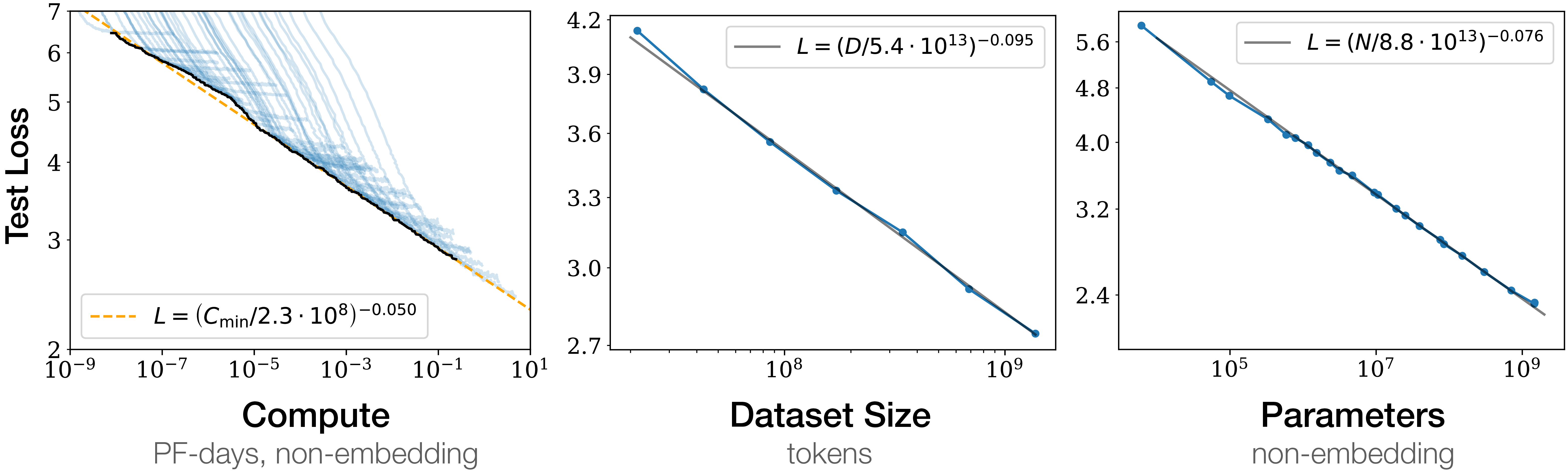
Neural scaling laws are simple predictive laws for how a model's performance (e.g. loss) scales with three key axes:

Model size (N): the number of parameters in the model
Dataset size (D): the number of training tokens
Compute (C): the total amount of computation used during training, measured in FLOPs or GPU-days

What is a GPU?

A GPU (Graphics Processing Unit) is a specialized processor built for massively parallel computation
It can execute thousands of simple operations at once, which makes it ideal for training neural networks
Modern AI training relies on large clusters of GPUs working together

What is a PF-day?

A FLOP (Floating Point Operation) is a single arithmetic operation of a floating-point number
A PF-day (petaFLOP/s day) is the compute from running at \(10^{15}\) FLOPs for 24h

\[ \begin{align} 1 \text{ PF-day} &= 10^{15} \text{ FLOP/s} \cdot 1 \text{ day} \\ &= 10^{15} \text{ FLOP/s} \cdot 60 \cdot 60 \cdot 24 s \\ &= 8.64 \cdot 10^{19} \text{ FLOP} \end{align} \]

GPT-3 (175B params) cost ~\(3,640\) PF-days to train (2020)

A V100 GPU delivers ~\(28 \times 10^{12}\) FLOP/s (bf16)

\(1 \text{ PF-day} = \frac{10^{15} \text{ FLOP/s} \cdot \text{ day}}{28 \cdot 10^{12} \text{ FLOP/s/GPU}} \approx 36 \text{ GPU-days}\)

GPT-3 training would require ~\(3,640 \cdot 36 = 131,040 \text{ GPU-days}\)

Brown et al., Language Models are Few-Shot Learners, arXiv:2005.14165 (2020)

OpenAI's GPT-3 Language Model: A Technical Overview, link (2020)

FLOPs in a Matrix-Vector Multiply

\[ \sum_{j=1}^{d} W_{ij}\, x_j = y_i \]

\[ \underbrace{\begin{bmatrix} W_{11} & \cdots & W_{1d} \\ \vdots & \ddots & \vdots \\ W_{H1} & \cdots & W_{Hd} \end{bmatrix}}_{H \times d} \underbrace{\begin{bmatrix} x_1 \\ \vdots \\ x_d \end{bmatrix}}_{d \times 1} = \underbrace{\begin{bmatrix} y_1 \\ \vdots \\ y_H \end{bmatrix}}_{H \times 1} \]

\[ y_1 = W_{11} x_1 + W_{12} x_2 + \cdots + W_{1d} x_d\] \(\text{FLOP}\) for one element of \(y\): \( d \) multiplies and \( d - 1 \) adds \( \approx 2d \)

\(\text{FLOP}\) per forward pass \(\approx 2 \cdot d \cdot H = 2N\)

Where \(N = dH\) (total parameters in the weight matrix)

Training Compute Derivation

\[ \underbrace{C}_{\text{Total FLOPs}} \approx \underbrace{2ND}_{\text{Forward Pass}} + \underbrace{4ND}_{\text{Backward Pass}} = 6ND \]

Forward Pass (\(2ND\)): One matrix-vector multiply per token (\(d\) multiplies + \(d\) adds) for each of the \(N\) parameters across \(D\) datapoints.
Backward Pass (\(4ND\)): Approximately 2x the compute of the forward pass.
- \(2ND\) to calculate gradients with respect to activations (\(\nabla x\)).
- \(2ND\) to calculate gradients with respect to weights (\(\nabla W\)).

\[ \boxed{C \approx 6ND} \]

Early Neural Network scaling

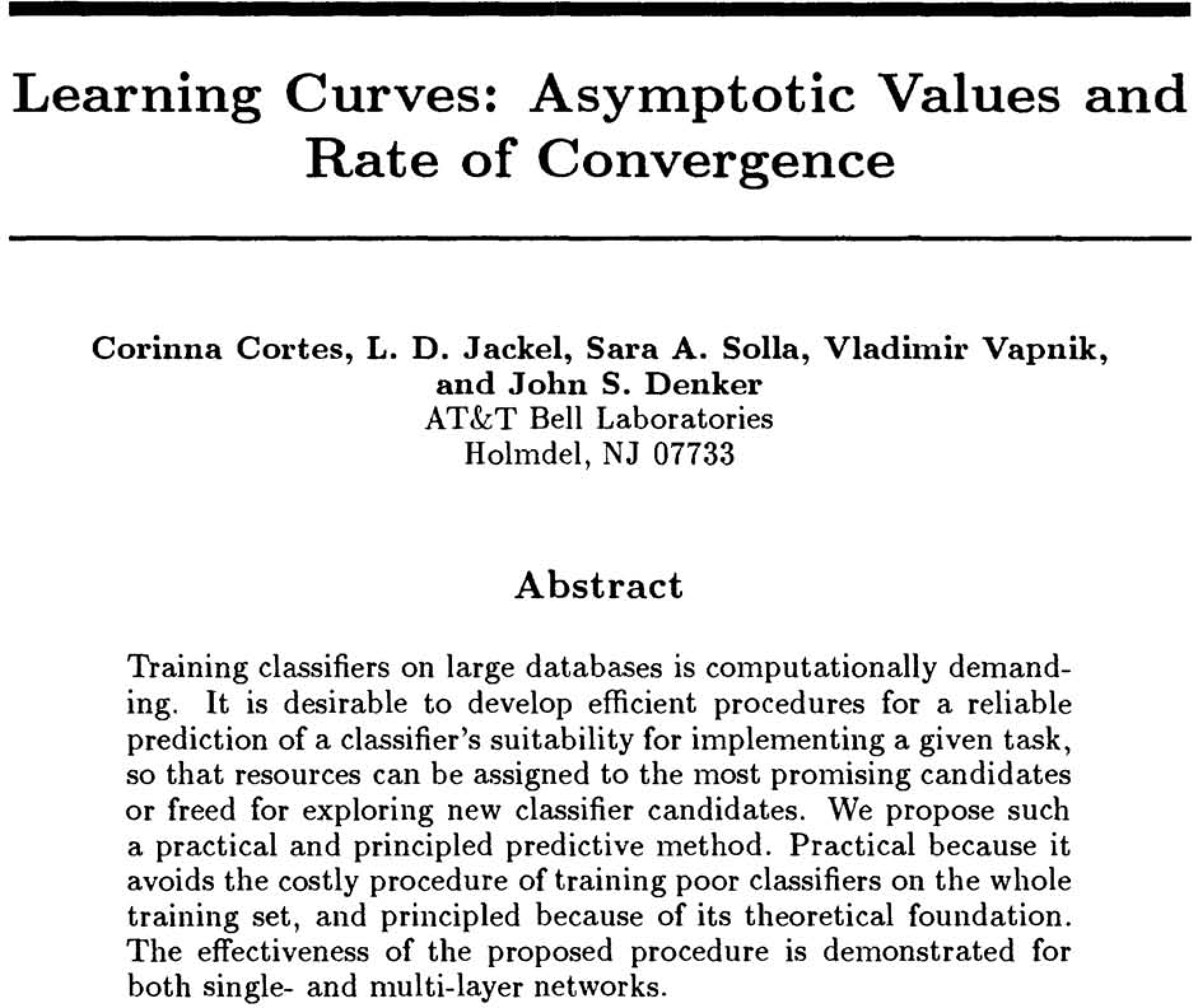
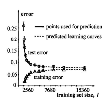
Takeaway: learning curves showed early evidence of power-law behavior decades before modern LLMs.

Amari et al., Learning Curves - Asymptotic Values and Rates of Convergence, NeurIPS, 1993

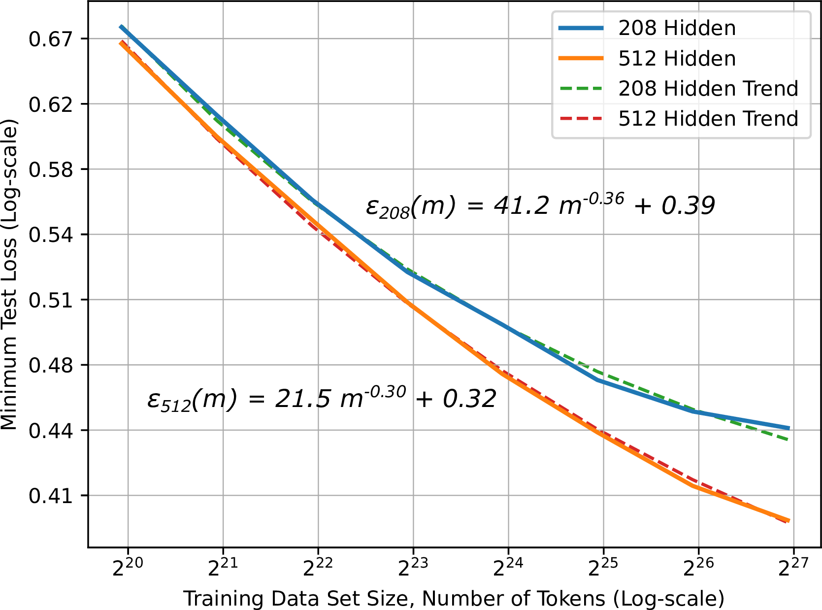
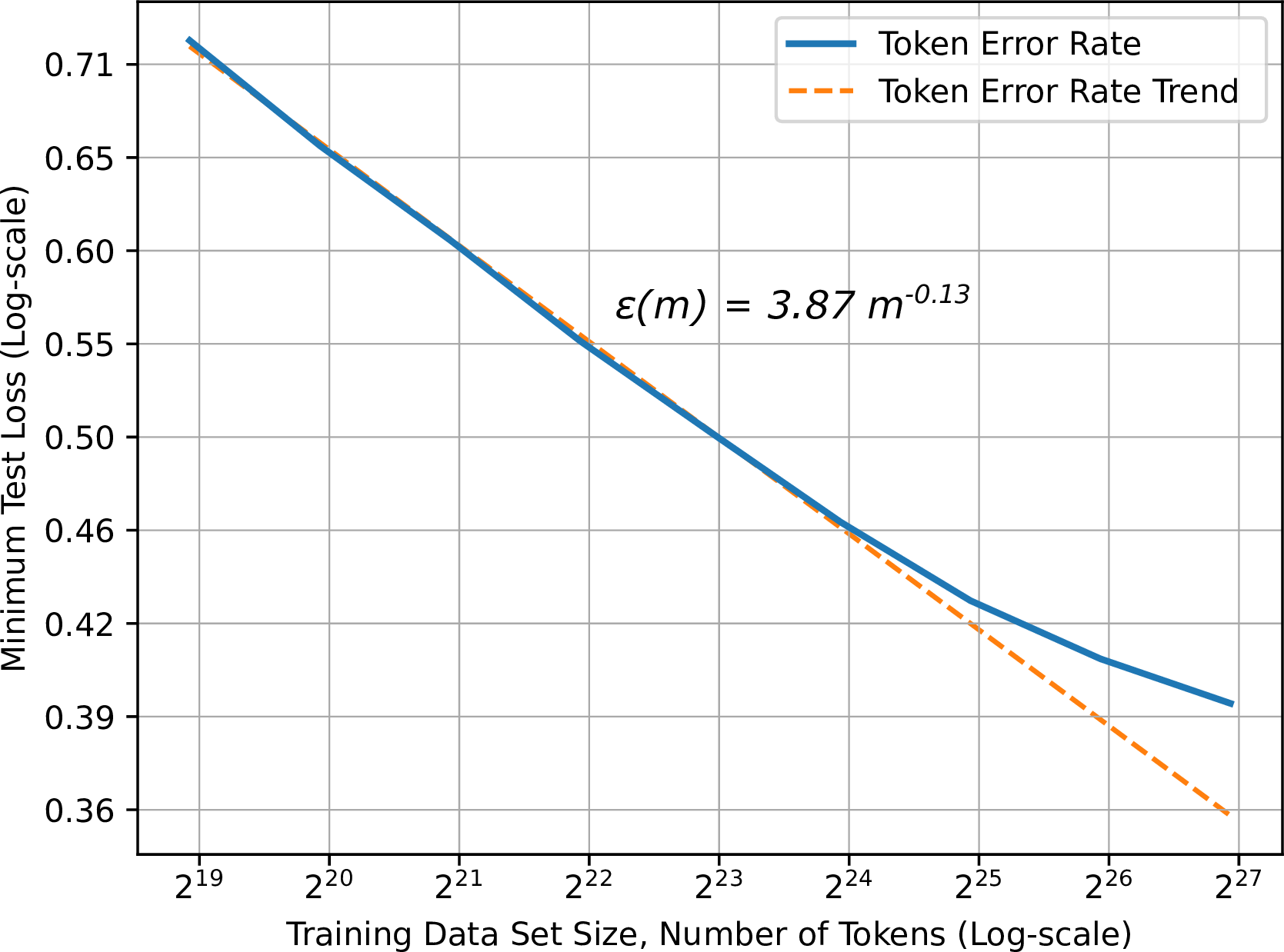
Deep Learning Scaling is Predictable, Empirically - Part 1

Machine translation error models — Figure: Neural machine translation learning curves.

Left: the learning curves for separate models follow \(\varepsilon(m) = \alpha m^{\beta_g} + \gamma\).

Right: composite learning curve of best-fit model at each data set size.

Machine translation generalization — Figure: Neural machine translation learning curves.

Left: the learning curves for separate models follow \(\varepsilon(m) = \alpha m^{\beta_g} + \gamma\).

Right: composite learning curve of best-fit model at each data set size.

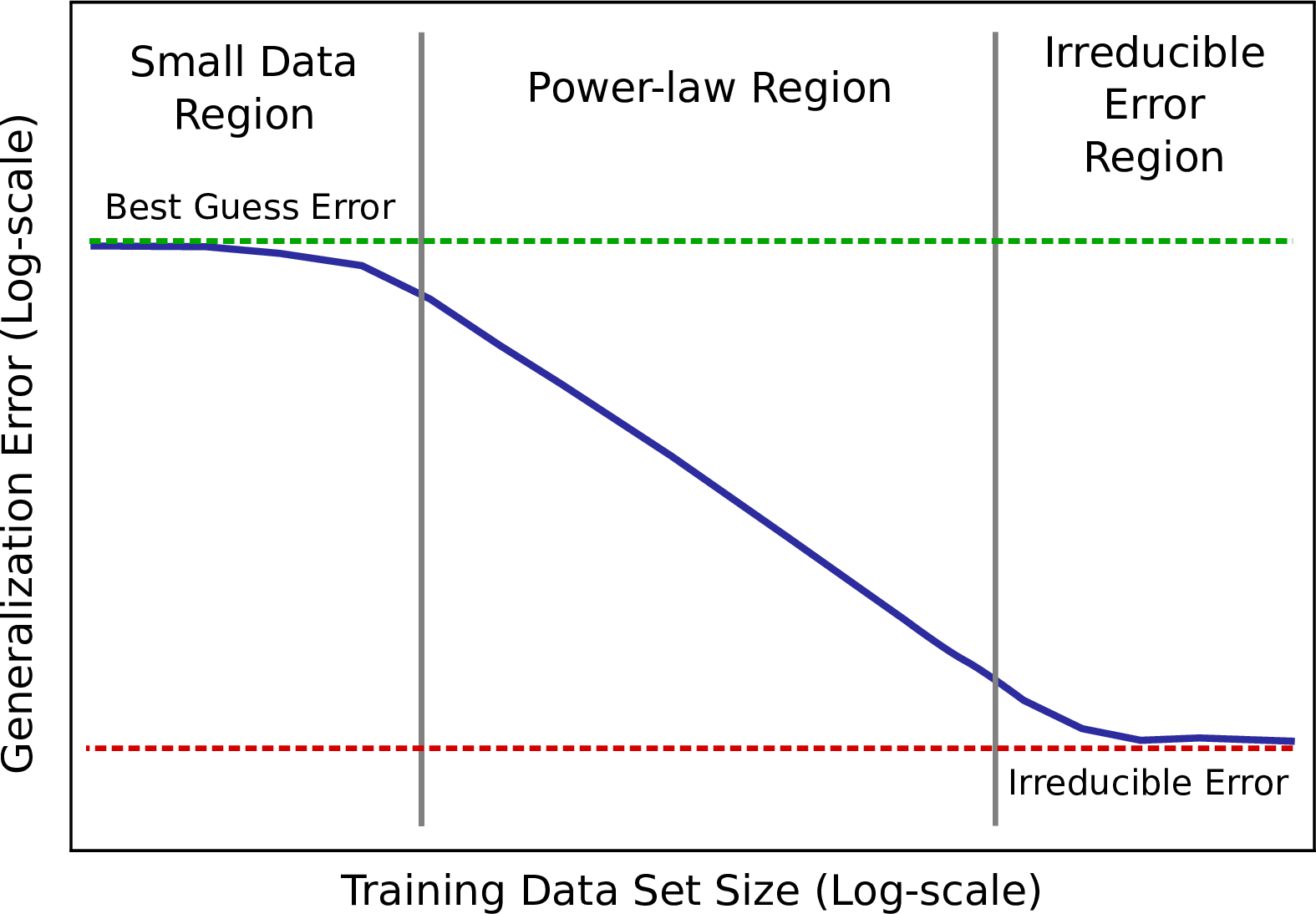
Takeaway: error scales predictably with data across tasks; power-law regions emerge.

Hestness et al., Deep Learning Scaling is Predictable, Empirically, arXiv:1712.00409 (2017)

Deep Learning Scaling is Predictable, Empirically - Part 2

Hestness et al., Deep Learning Scaling is Predictable, Empirically, arXiv:1712.00409 (2017)

EfficientNet (2019)

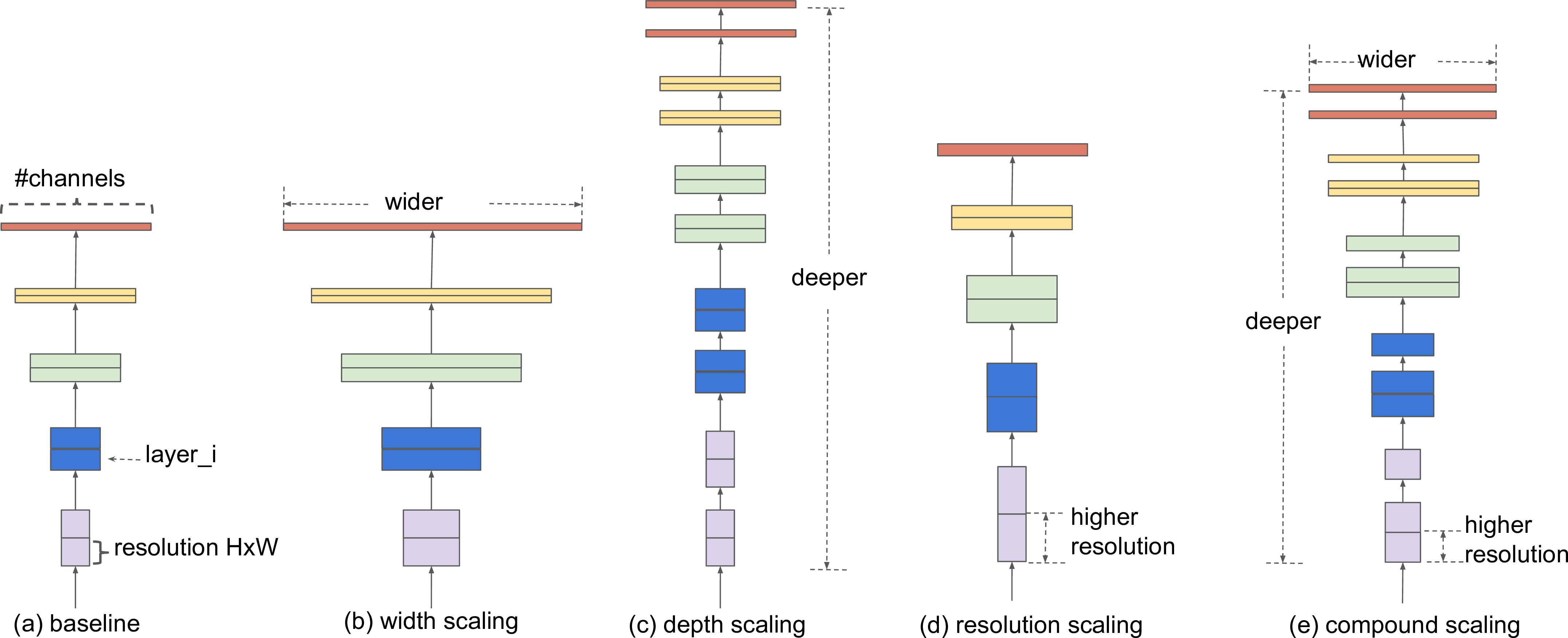
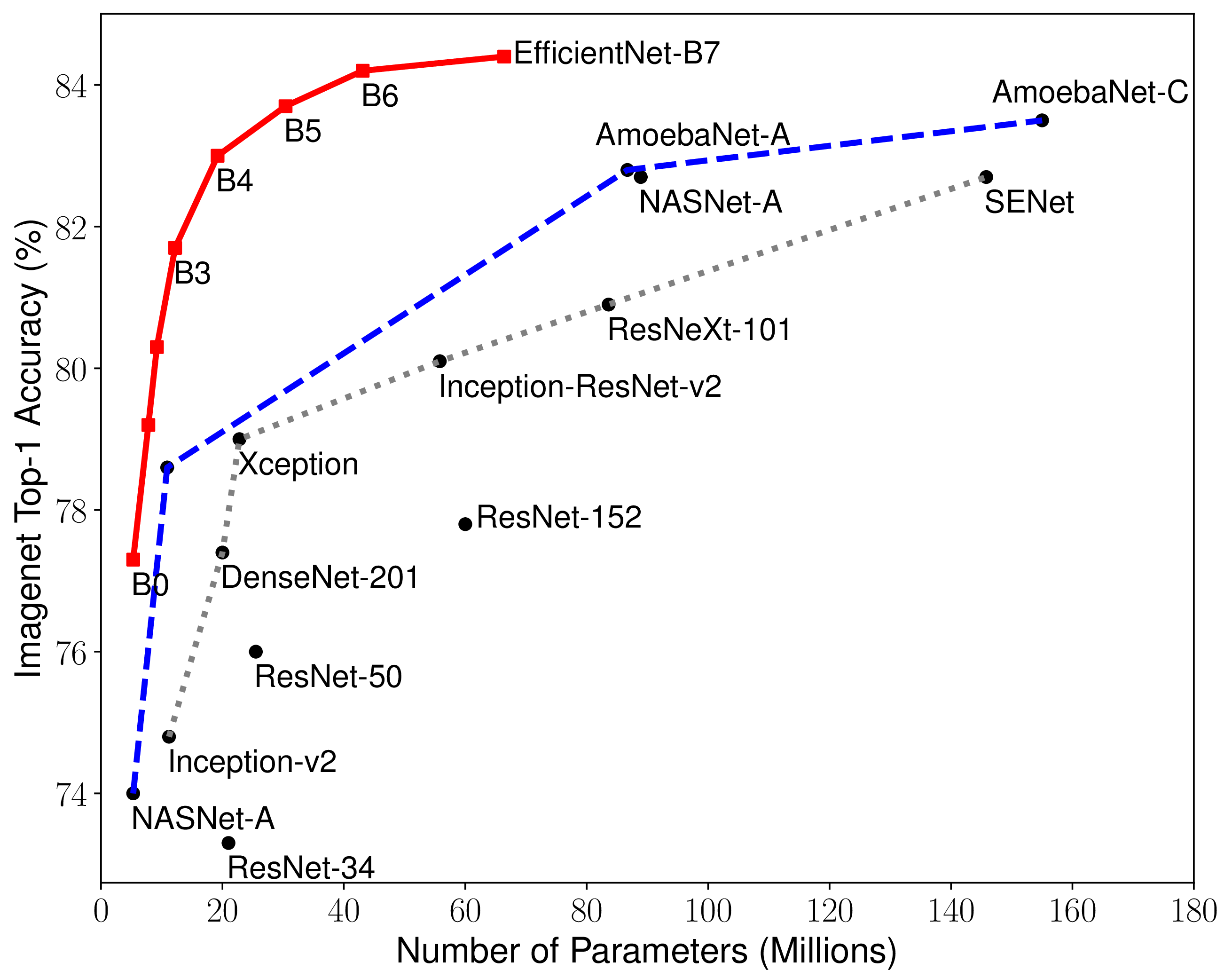
There are many ways to scale models, what is the optimal approach?

Performance is measured by the ImageNet classification error rate.

Fixed amount of training data is considered.

Tan and Le, EfficientNet: Rethinking Model Scaling for Convolutional Neural Networks arXiv:1905.11946

Scaling Laws for Neural Language Models (2020)

It's crucial in each case that all of the other quantities are much larger. For example, for model size scaling, we must have a very large dataset.

These are results when only one of \(N, D, C\) is bottlenecking performance.

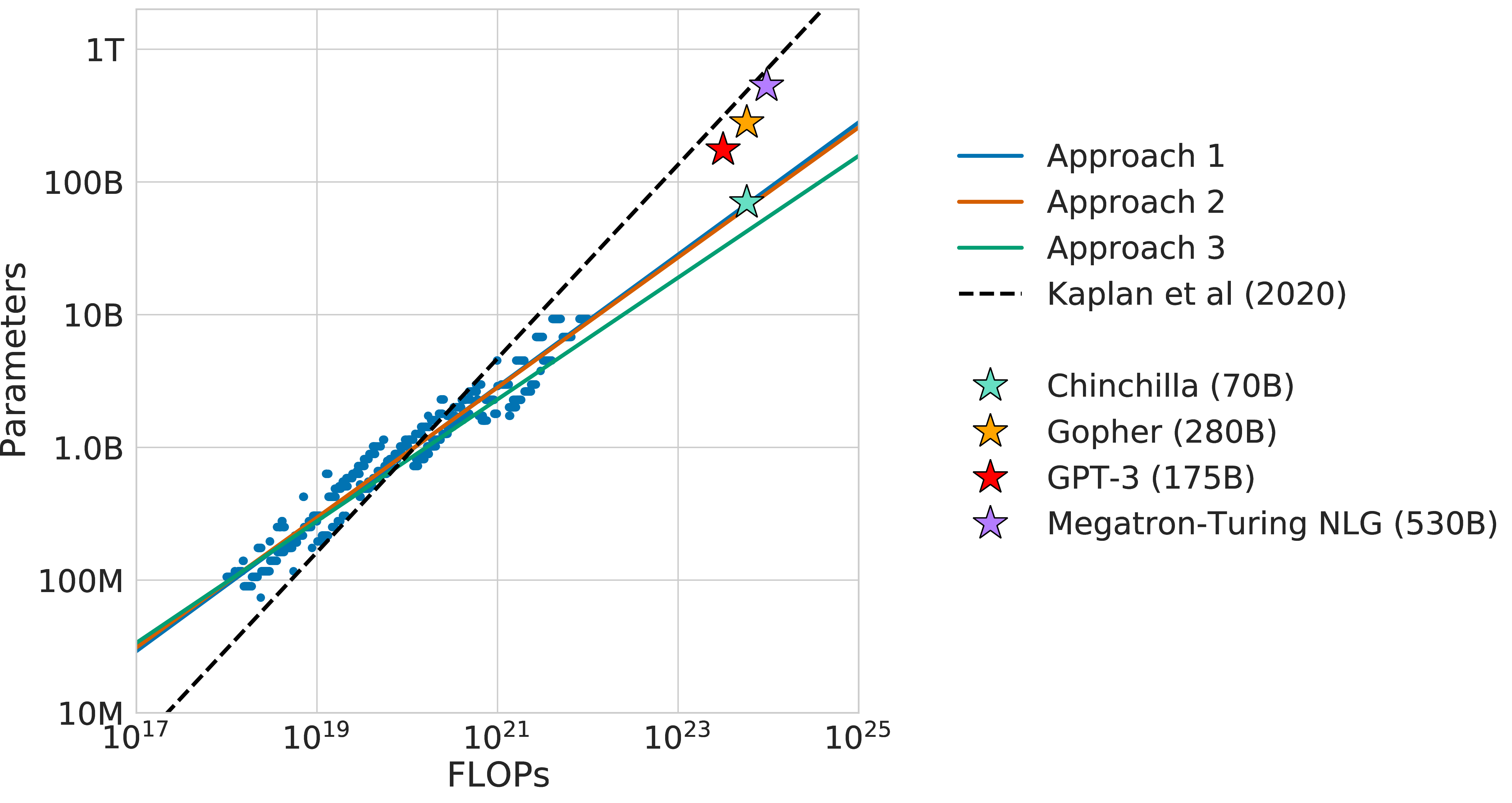
Kaplan et al., Scaling Laws for Neural Language Models, arXiv:2001.08361 (2020)

Training Compute-Optimal Large Language Models (2022)

Compute-optimal training balances model size and training tokens
Rule: for every doubling of parameters, double the number of training tokens
Trained 400+ models (70M-16B params) on 5-500B tokens to fit the scaling relationship
Chinchilla (70B) used the same compute as Gopher (280B) but trained on ~4x more data and outperformed across many tasks

Chinchilla compute-optimal predictions comparison

Hoffmann et al., Training Compute-Optimal Large Language Models, arXiv:2203.15556 (2022)

Training Stages

Pre-Training

Next-token prediction over large, diverse text
Builds broad knowledge and general representations
Scaling laws are most visible here

Fine-Tuning

Domain- or instruction-focused data
Refines behavior for specific use cases
Bridges pre-training and alignment

Post-Training

RLHF / RLVR and preference tuning
Optimize helpfulness, safety, and style

GPT-4 Predicted from Small Models

The scaling laws derived from smaller models were used to predict GPT-4's performance before its training.

OpenAI, GPT-4 Technical Report, arXiv:2303.08774 (2023)

Practice Leads Theory

Scaling laws were found empirically before we had a full theory
The field often advances by measuring first, then explaining later
Key question: why do simple power laws hold across so many regimes?

The Irreducible Floor of Language

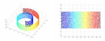
Imagine that the data lives on a low-dimensional manifold. The model must learn to navigate this space effectively.

\[ L(N,\,D) = E + \frac{A}{N^{\alpha}} + \frac{B}{D^{\beta}} \]

irreducible floor: E nats / token

Hoffmann et al., Training Compute-Optimal Large Language Models, arXiv:2203.15556 (2022) - Equation. (2)

Manifold Intuition

Data lives on a lower-dimensional manifold inside a high-dimensional space
More data means denser sampling of that manifold
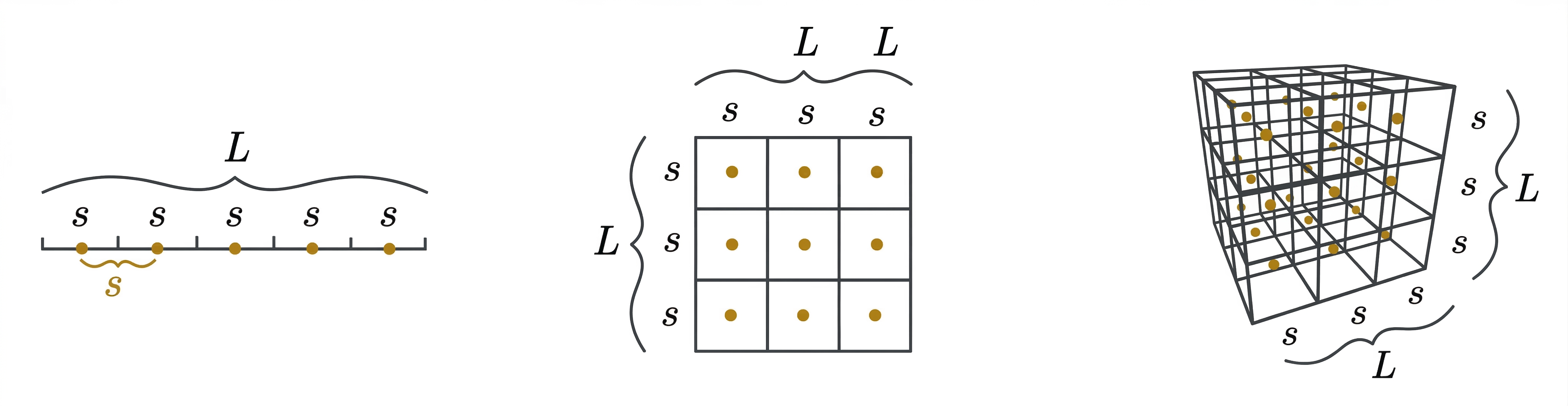
Power laws can emerge from geometric sampling effects

Image: Swiss roll manifold, a common example in machine learning to illustrate data lying on a low-dimensional manifold. scikit-learn documentation

Why do Scaling Laws hold?

1-dimensional manifold: \( s = L/D \) (distance between points).
2-dimensional manifold: \( L^2=D\cdot s^2\,\implies\, s = \sqrt{L^2/D}=L\cdot D^{-1/2} \)
3-dimensional manifold: \( s = L\cdot D^{-1/3} \)
d-dimensional manifold: \( s = L\cdot D^{-1/d} \)

Bahri et al., Explaining Neural Scaling Laws, arXiv:2102.06701 (2024)

Inference Changes the Equation

Scaling laws minimize training loss for fixed compute - they ignore inference cost
Inference is now the majority of total compute for deployed models
Smaller, more thoroughly trained models are cheaper overall at scale
As inference volume grows, the cost-optimal point shifts toward smaller models with more training tokens

GPT3 - 2 tokens / param
Chinchilla - 20 tokens / param
LLaMA65B - 22 tokens / param
Llama 2 70B - 29 tokens / param
Mistral 7B - 110 tokens / param
Llama 3 70B - 215 tokens / param

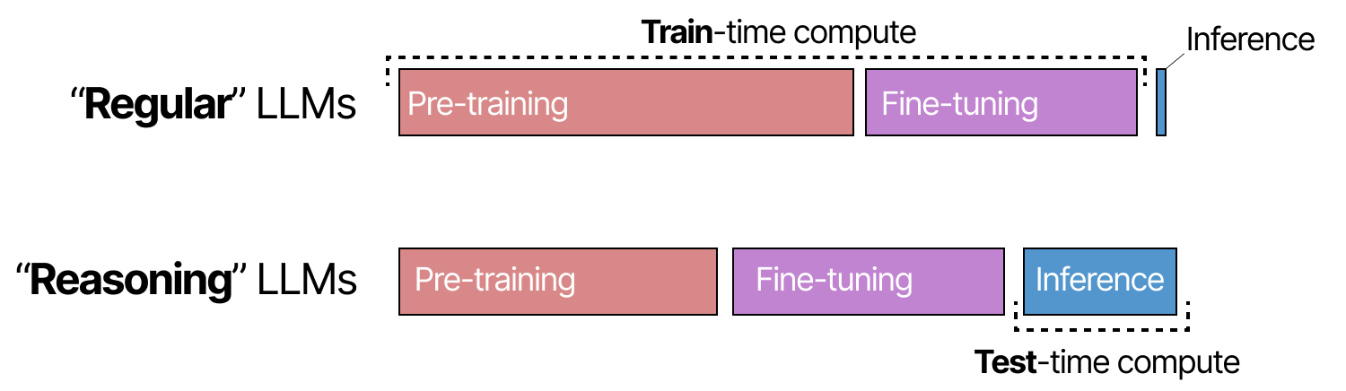
Inference-Time Compute

A third scaling axis: inference-time compute - longer chains -> better answers
Reasoning allows the model to use more compute for the same task

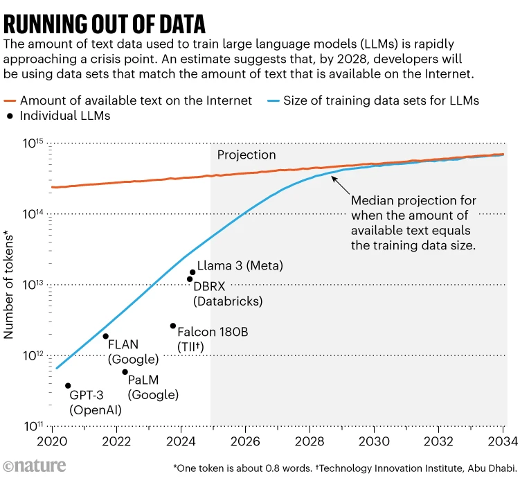
Maarten Grootendorst, A Visual Guide to Reasoning LLMs, maartengrootendorst.com (2025)

Wei et al., Chain-of-Thought Prompting Elicits Reasoning in Large Language Models, arXiv:2201.11903 (2022)

LLMs and the Data Bottleneck

Nature (2024), We're running out of data to train AI. nature.com

Villalobos et al., Will we run out of data? Limits of LLM scaling based on human-generated data, arXiv:2211.04325 (2024)

Task-Completion Time Horizons

METR, Task-Completion Time Horizons of Frontier AI Models, 2026, Source, Hosted Backup

The Bitter Lesson

"general methods that leverage computation are ultimately the most effective."

Richard Sutton, The Bitter Lesson, 2019, Source, Hosted Backup

Where are we going?

Scaling continues to yield improvements and has expanded to new axes beyond pre-training (RL, inference-time compute)
Use of less pre-generated data and more synthetic data and real-world interactions
Length of tasks AI handles autonomously doubling every ~7 months (METR 2025)